Simulations
LIME Toolbox allows users to simulate lunar reflectance, irradiance, the degree of linear polarisation (DoLP), and the angle of linear polarisation (AoLP). Simulations are performed using the Simulation page (Figure 6), which is the default view when launching LIME Toolbox.
Users can select one of three simulation methods:
Geographic Coordinates – Based on an Earth-based location.
Selenographic Coordinates – Based on a location on the Moon.
Satellite Position – Based on an orbiting satellite’s position.
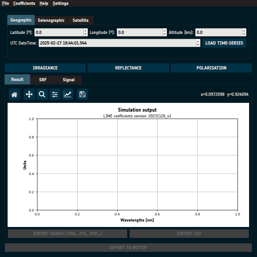
Figure 6: Simulation page.
Simulation Using Geographic Coordinates
Selecting the “Geographic” tab allows users to perform simulations based on Earth coordinates (Figure 7). Users must provide:
Latitude & Longitude (in decimal degrees)
Altitude (in kilometers)
UTC Date & Time
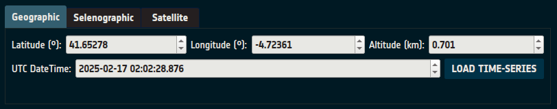
Figure 7: Geographic coordinates input.
Time-Series Input
For multiple timestamps, click “LOAD TIME-SERIES”, which enables time-series file input (Figure 8).
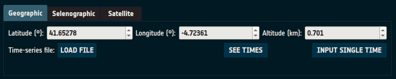
Figure 8: Geographic coordinates input for multiple timestamps.
Loading Time-Series Data
Click “LOAD FILE” to open a file selection dialog.
Select a file containing timestamps in one of the following formats:
ISO 8601 format
Comma-separated values (CSV):
yyyy,mm,dd,HH,MM,SSyyyy,mm,dd,HH,MM,SS,microseconds
Example Valid File
2022,01,17,02,02,04
2023,01,17,02,02,04,123545
2020-01-12 00:22:43.124
Additional options:
“SEE TIMES” – Opens a window displaying imported timestamps.
“INPUT SINGLE TIME” – Switches back to single timestamp mode.
Command-Line Interface (CLI)
Use the -e or --earth option:
lime -e latitude_deg,longitude_deg,height_km,datetime_isoformat
Example
For a simulation of 35° of latitude, -25.2° of longitude, 400 meters of altitude, and at the date and time of 2022-01-20 02:00:00 UTC:
lime -e 35,-25.2,0.4,2022-01-20T02:00:00
For time-series input:
lime -e 35,-25.2,0.4 -t timeseries.txt
Simulation Using Selenographic Coordinates
Selecting the “Selenographic” tab enables simulations using Moon-based coordinates (Figure 9). Users must provide:
Sun-Moon Distance (AU)
Observer-Moon Distance (km)
Selenographic Latitude & Longitude of Observer (decimal degrees)
Selenographic Longitude of the Sun (decimal degrees)
Moon Phase Angle (decimal degrees)
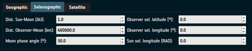
Figure 9: Selenographic coordinates input.
Multiple Points Input
You can load several selenographic coordinates at once instead of entering them individually.
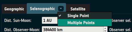
Figure 10: Selenographic tab’s dropdown menu, with Multiple Points option highlighted.
Open the Selenographic tab’s dropdown menu and select Multiple Points (Figure 10).
The multiple selenographic input page will appear (Figure 11). Click “LOAD FILE” and choose a
.csvfile containing the coordinates.
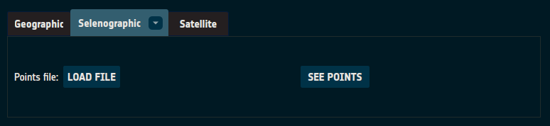
Figure 11: Multiple selenographic points input page.
The file should have one point per line, with six comma-separated values in the following order:
sun_moon_distance_au,observer_moon_distance_km,observer_selenographic_latitude_deg,observer_selenographic_longitude_deg,solar_selenographic_longitude_deg,moon_phase_angle_deg
Command-Line Interface (CLI)
Use the -l or --lunar option to run a lunar simulation. You can provide the input parameters in two ways:
1. Single simulation (inline):
lime -l distance_sun_moon,distance_observer_moon,selen_obs_lat,selen_obs_lon,selen_sun_lon,moon_phase_angle
Example
For a simulation for 0.98 AU of Sun-Moon Distance, 420000 km of Observer-Moon Distance, 20.5° and -30.2° as the selenographic latitude and longitude of the observer, 69° as the selenographic longitude of the Sun, and 15° as the moon phase angle:
lime -l 0.98,420000,20.5,-30.2,69,15
2. Batch simulation (.csv file):
lime -l multiple_points.csv
The .csv file must follow the exact same format described in the
Multiple Points Input section above (same column names and order).
Simulation Using Satellite Positions
Selecting the “Satellite” tab enables simulation based on orbiting satellites (Figure 12).
Users must:
Select a satellite from the available list.
Provide a UTC Date & Time.
Note: Time-series input works the same as in Geographic Coordinates.
Selecting the “Satellite” tab enables simulations based on orbiting satellite (Figure 12). Users must:
Select a satellite from the available list.
Provide a UTC Date & Time.
Note: Time-series input works the same as in Geographic Coordinates.
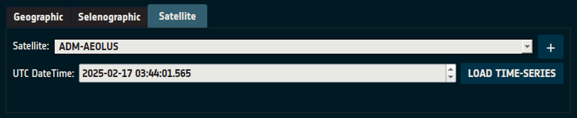
Figure 12: Satellite position input.
Adding a New Satellite
It’s possible to add user-defined satellites to the list of available satellites.
Click the button with a plus (+) sign on the right of the dropdown.
The user will be prompted with the Add Satellite Data window (Figure 13).
Click “LOAD FILE” which opens a file selection dialog where users can load Orbit Scenario Files (OSF) or Three-Line Element Set files (TLE/3LE).
The Add Satellite Data window will now display information of the loaded file, and the user must fill the last details.
Satellite Name: Only editable for OSF files. Name that will be displayed in the satellite list.
Start time: Date when the file validity starts.
End time: Date when the file validity stops.
Click “SAVE SATELLITE DATA” to store the loaded data in the local LIME Toolbox system.
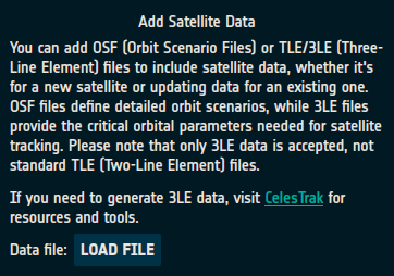
Figure 13: Add Satellite Data window.
Command-Line Interface (CLI)
Use the -s or --satellite option:
lime -s sat_name,datetime_isoformat
Example
To perform a simulation for the satellite PROVA-B at the date and time of 2020-01-20 02:00:00h:
lime -s PROBA-V,2020-01-20T02:00:00
As in Geographic Coordinates, one can use time-series input:
lime -s PROBA-V -t timeseries.txt
It’s not possible to add a user-defined satellite throught the CLI at the moment.
Simulation output
The simulation results are displayed below the input section. Users can select one of the following button to run simulations and view results:
“IRRADIANCE” – Displays irradiance results.
“REFLECTANCE” – Shows reflectance results.
“DOLP” – Visualises the Degree of Linear Polarisation (DoLP).
“AOLP” – Visualises the Angle of Linear Polarisation (AoLP).
These buttons are positioned between the input and the output, as shown on top of Figure 14.
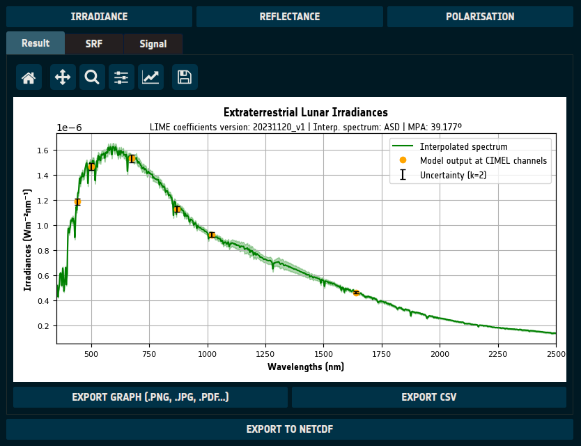
Figure 14: Simulation output.
Results are plotted with:
X-axis → Wavelengths.
Y-axis → Computed values.
Exporting Simulation Results
Users can export the results in multiple formats:
Graphical Export (Image/PDF)
Click “Export Graph” (top-center) to save the graph as an image or PDF.
A file system dialog will prompt the user to select the location, filename, and format.
Supported formats include JPG, PNG, PDF, and other common image formats.
Data Export (CSV File)
Click “Export CSV” (top-center) to save the simulation data as a comma-separated values (CSV) file.
The user will be prompted to choose the location and filename.
NetCDF Export
Go to the action menu bar and navigat to “File → Save as a netCDF file” to save results as a netCDF file.
Why use netCDF?
Unlike CSV, netCDF allows LIME Toolbox to reload previous simulations for visualization.
This format enables efficient data storage and retrieval.
Command-Line Interface (CLI) Export Options
In the CLI, results are only accessible by exporting them to data files.
To do this, users must utilize the -o or --output option, with the argument varying
based on the desired output type.
Graphical Export (Image/PDF)
Specify the image type, paths and filenames of each graph:
-o graph,(pdf|jpg|png|svg),reflectance_path,irradiance_path,dolp_path,aolp_path
For example:
-o graph,jpg,reflectance.jpg,irradiance.jpg,dolp.jpg,aolp.jpg
Data Export (CSV File)
Specify paths and names of each file:
-o csv,reflectance_path,irradiance_path,dolp_path,aolp_path,integrated_irradiance_path
For example:
-o csv,reflectance.csv,irradiance.csv,dolp.csv,aolp.csv,integrated_irradiance.csv
NetCDF Export
Specify the netCDF file path:
-o nc,output_path
For example:
-o nc,output.nc
Integrated Irradiance
LIME Toolbox integrates the calculated irradiance over the selected spectral response function (SRF). These values appear in the “Signal” tab (Figure 15), showing one value per SRF channel, and can be exported as CSV.
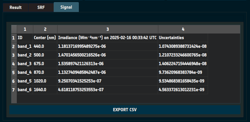
Figure 15: Signal tab showing some results for the CIMEL SRF.
Spectral Response Functions (SRF)
Users can visualise, load, and switch between different SRFs in the “SRF” tab (Figure 16). This tab presents:
A graph of the currently selected SRF, where:
X-axis represents wavelengths.
Y-axis represents the spectral response.
Two vertical black lines marking the lower and upper simulation limits of LIME Toolbox.
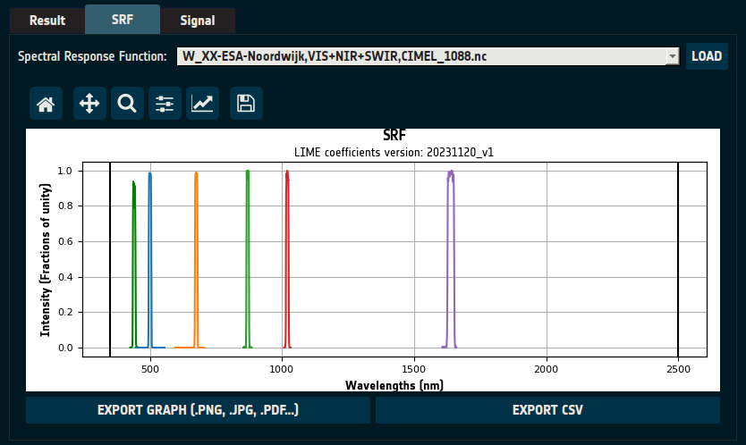
Figure 16: SRF tab showing CIMEL SRF.
By default, LIME Toolbox includes a default SRF that encompasses the entire LIME spectrum, named “Default”.
Loading a New SRF
Click “LOAD” (top-right corner in Figure 16).
Select a netCDF SRF file in GLOD format (explained in the File Formats section).
Once loaded, use the dropdown menu next to the “LOAD” button to switch between SRFs.
This can also be done in the CLI using the -f or --srf option followed by the SRF path:
-f srf_path
Exporting SRF Data
Graphs can be exported as images or PDFs.
SRF data can be exported as CSV files.